Rectified LpJEPA
Joint-Embedding Predictive Architectures with Sparse and Maximum-Entropy Representations
Introduction
This post is a companion blog to our paper Rectified LpJEPA (arXiv:2602.01456 ) and its accompanying implementation (GitHub ). The goal is to provide a self-contained walkthrough of the key ideas in a less technical manner.
We begin by reviewing self-supervised learning and the problem of feature collapse, then motivate distribution-matching regularization through the Cramér–Wold theorem and its instantiation in SIGReg / LeJEPA
Self-Supervised Learning
Consider an input vector $\mathbf{x}$, such as an image, an audio clip, or a video frame. We would like to learn a neural network representation
\[\begin{align} \mathbf{z}=f_{\boldsymbol{\theta}}(\mathbf{x})\in\mathbb{R}^d \tag{1} \end{align}\]in the absence of any labeling information, where \(f_{\boldsymbol{\theta}}(\cdot)\) is the neural network with parameters \(\boldsymbol{\theta}\). Self-supervised learning makes this possible by creating supervision from the data itself
- For images, $\mathbf{x}'$ might be a cropped, rotated, or even corrupted version of $\mathbf{x}$
- For audio or video, $\mathbf{x}'$ can be a nearby time segment or adjacent frame.
Although $\mathbf{x}$ and $\mathbf{x}'$ may look different, they are assumed to be semantically related. Thus we can learn a neural network representation by relying on the following principle: representations of different views of the same input should be similar. Translating to mathematical language, this means we can minimize the $\ell_2$ distance between the embeddings of different views
\[\begin{align} \min_{\boldsymbol{\theta}}\mathbb{E}_{\mathbf{z},\mathbf{z}'}[\|\mathbf{z}-\mathbf{z}'\|_2] \tag{2} \end{align}\]where \(\mathbf{z}' = f_{\boldsymbol{\theta}}(\mathbf{x}')\) and \(\mathbf{z}'\sim\mathbb{P}_{\mathbf{z}'}\), \(\mathbf{z}\sim\mathbb{P}_{\mathbf{z}}\) are sampled from the feature distributions. By enforcing agreement across many randomly generated views, the network learns features that are invariant to nuisance transformations and capture meaningful structure in the data.
Distribution-Matching Regularization
Distribution-Matching as Regularization
Simply minimizing the \(\ell_2\) distance (Eq. (2)) between views, however, can lead to the problem of feature collapse. In the extreme case, the network can map every input to the same vector, resulting in complete collapse. Eq. (2) is perfectly minimized, but the representation is useless as it cannot distinguish between different inputs. More subtle forms of collapse also occur, such as dimensional collapse, where different feature dimensions encode redundant information
The goal of self-supervised learning is therefore to enforce invariance across views while maximally spreading feature vectors in the ambient space to prevent collapse. One effective way to do this is to regularize the feature distributions \(\mathbb{P}_{\mathbf{z}}\) and \(\mathbb{P}_{\mathbf{z}'}\) towards a carefully chosen target distribution \(Q\), which explicitly encodes desirable properties such as dispersion and diversity across feature dimensions. Thus the self-supervised learning objective in Eq. (2) can be augmented as
\[\begin{align} \min_{\boldsymbol{\theta}}\mathbb{E}_{\mathbf{z},\mathbf{z}'}[\|\mathbf{z}-\mathbf{z}'\|_2]+\mathcal{L}(\mathbb{P}_{\mathbf{z}}\|Q)+\mathcal{L}(\mathbb{P}_{\mathbf{z}'}\|Q) \tag{3} \end{align}\]where \(\mathcal{L}(P\|Q)\) is any differentiable distributional discrepancy that is minimized when \(P\) and \(Q\) are equal in distribution.
Naively, one can consider the KL divergence \(D_{\operatorname{KL}}(\mathbb{P}_{\mathbf{z}}\|Q)\) with the Monte-Carlo estimate:
\[\begin{align} D_{\operatorname{KL}}(\mathbb{P}_{\mathbf{z}}\|Q) = \int\log\frac{d\mathbb{P}_{\mathbf{z}}(\mathbf{z})}{dQ(\mathbf{z})}d\mathbb{P}_{\mathbf{z}}(\mathbf{z})\approx \frac{1}{B}\sum_{i=1}^{B}\log\frac{p_{\mathbf{z}}(\mathbf{z}_i)}{q(\mathbf{z}_i)} \tag{4} \end{align}\]However, directly performing distribution-matching in high dimensional space suffers from the curse of dimensionality: density estimations are intractable and we require exponential number of samples in dimensions
Cramér-Wold Theorem
The Cramér-Wold theorem states that two random vectors \(\mathbf{x},\mathbf{y}\in\mathbb{R}^d\) are equal in distribution if and only if all of their one-dimensional projected marginals are equal in distribution, i.e.
\[\begin{align} \mathbf{x}\stackrel{\operatorname{d}}{=}\mathbf{y}\iff \mathbf{c}^\top\mathbf{x}\stackrel{\operatorname{d}}{=}\mathbf{c}^\top\mathbf{y}\text{ for all }\mathbf{c}\in\mathbb{R}^d \tag{5} \end{align}\]where the superscript \(\operatorname{d}\) above the equal sign denotes equality in distribution. This result enables us to decompose a high-dimensional distribution matching problem into parallelized one-dimension optimizations under many different projections induced by \(\mathbf{c}\), which significantly reduces the sample complexity in each of the one-dimensional problems. This projection-based distribution matching idea traces back to projection pursuit. See
With the Cramér–Wold theorem, Eq. (3) can be updated as
\[\begin{align} \min_{\boldsymbol{\theta}}\mathbb{E}_{\mathbf{z},\mathbf{z}'}[\|\mathbf{z}-\mathbf{z}'\|_2]+\mathbb{E}_{\mathbf{c}}[\mathcal{L}(\mathbb{P}_{\mathbf{c}^\top\mathbf{z}}\|\mathbb{P}_{\mathbf{c}^\top\mathbf{y}})]+\mathbb{E}_{\mathbf{c}}[\mathcal{L}(\mathbb{P}_{\mathbf{c}^\top\mathbf{z}'}\|\mathbb{P}_{\mathbf{c}^\top\mathbf{y}})] \tag{6} \end{align}\]where \(\mathbf{y}\sim Q\), \(\mathbf{c}^\top\mathbf{y}\sim\mathbb{P}_{\mathbf{c}^\top\mathbf{y}}\) denotes the distribution of the projected targets, and \(\mathbf{c}^\top\mathbf{z}\sim\mathbb{P}_{\mathbf{c}^\top\mathbf{z}}\) represents the distribution of the projected features. Thus we have converted a high-dimensional distribution matching problem \(\mathcal{L}(\mathbb{P}_{\mathbf{z}}\|Q)\) into an expectation over univariate distribution-matching objectives as \(\mathbb{E}_{\mathbf{c}}[\mathcal{L}(\mathbb{P}_{\mathbf{c}^\top\mathbf{z}}\|\mathbb{P}_{\mathbf{c}^\top\mathbf{y}})]\).
Even if Cramér–Wold theorem guarantees convergence under asymptotic number of projection vectors, in practice we only need finite projections and it suffices to sample the projection vectors \(\mathbf{c}\) uniformly from the unit \(\ell_2\) sphere \(\mathbb{S}^{d-1}_{\ell_2}:=\{\mathbf{x}\in\mathbb{R}^{d}\mid\|\mathbf{x}\|_2=1\}\), rather than from the entire space \(\mathbb{R}^d\)
Sketched Isotropic Gaussian Regularization (SIGReg)
The SIGReg objective in LeJEPA
where \(\varphi_{P}\) denotes the characteristic function of the distribution \(P\) and \(\omega(t)=e^{-t^2/2}\) is the weight function. Intuitively, SIGReg minimizes the discrepancy between the characteristic function of the projected features—estimated empirically from minibatch samples—and that of the projected target distribution, which admits a closed-form expression.
This formulation yields a one-sample goodness-of-fit test: only the feature distribution is estimated from data, while the target distribution is fixed and analytically specified through its characteristic function. As we show later, the RDMReg loss for our Rectified LpJEPA requires a two-sample goodness-of-fit test due to a different choice of the target distribution \(Q\).
Target Distributions
In the following section, we discuss choices of the target distribution \(Q\) that encourage maximally spread-out and diverse feature representations, while simultaneously encoding sparsity. We begin, however, by revisiting the isotropic Gaussian, which induces dense representations and serves as a natural baseline.
Isotropic Gaussian Distributions
One natural target distribtuion is the isotropic Gaussian \(\mathcal{N}(\mathbf{0},\mathbf{I}_{d})\), which is used in LeJEPA
Probability Density Functions of Isotropic Gaussian
\[p(\mathbf{z})=\frac{1}{(2\pi)^{d/2}}\exp\bigg(-\frac{1}{2}\|\mathbf{z}\|_2^2\bigg)\]
The choice of Gaussian as the target distribution is not an arbitrary one. Geometrically, a $d$-dimensional isotropic Gaussian random vector $\mathbf{z}\sim\mathcal{N}(\mathbf{0},\mathbf{I}_{d})$ concentrates on a thin shell of radius $\sqrt{d}$ with an $O(1)$ width. Under polar decompositions, the radius $||\mathbf{z}||_2\sim\chi(d)$ and the angular direction $\mathbf{z}/||\mathbf{z}||_2$ are independent, with the direction uniformly distributed over the unit $\ell_2$ sphere with respect to the surface (Hausdorff) measure. This uniform angular distribution coincides exactly with the uniformity condition identified as optimal for contrastive learning
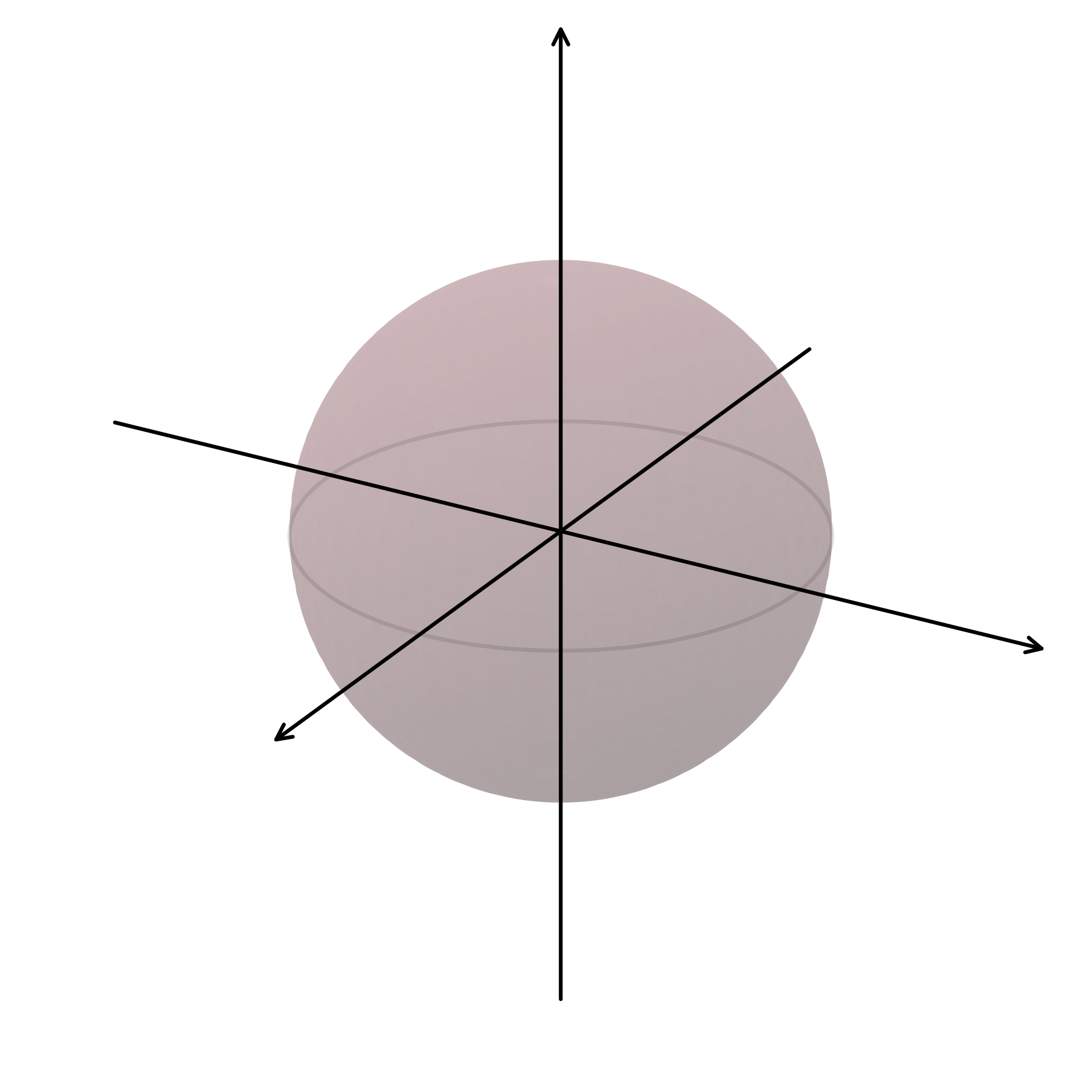
This geometric behavior has a direct information-theoretic correspondence. Among all possible probability distributions with a fixed expected $\ell_2$-norm (i.e., fixed average energy), the isotropic Gaussian maximizes entropy. In other words, if we constrain only how much energy the features carry and impose no further structure, the Gaussian is the most “spread out” distribution possible.
Product Laplace Distributions
While isotropic Gaussian regularization effectively prevents feature collapse, it inherently favors dense representations, where most feature dimensions are active. In contrast, extensive evidence from neuroscience, signal processing, and machine learning suggests that sparse representations are often more efficient and robust. Sparse coding plays a central role in compressed sensing and robust recovery, and biological neural systems are known to encode sensory inputs using non-negative, sparse activations under metabolic constraints
Motivated by these observations, we seek to induce sparsity directly at the level of the feature distribution. A simple and principled approach is to replace isotropic Gaussian regularization with product Laplace \(\prod_{i=1}^{d}\mathcal{L}(0,\sigma)\) regularization.
Probability Density Functions of Product Laplace
\[p(\mathbf{z})=\frac{1}{(2\sigma)^d}\exp\bigg(-\frac{\|\mathbf{z}\|_1}{\sigma}\bigg)\]
Contrary to Gaussian, the product Laplace distribution \(\mathbf{z}\sim\prod_{i=1}^{d}\mathcal{L}(0,\sigma)\) is the maximum-entropy distribution under a fixed expected $\ell_1$-norm constraint. Its radius follows the Gamma distribution \(\|\mathbf{z}\|_1\sim\Gamma(d/1, 1)\) and the angular direction \(\mathbf{z}/\|\mathbf{z}\|_1\) is uniformly distributed over the unit $\ell_1$ sphere with respect to the surface measure.
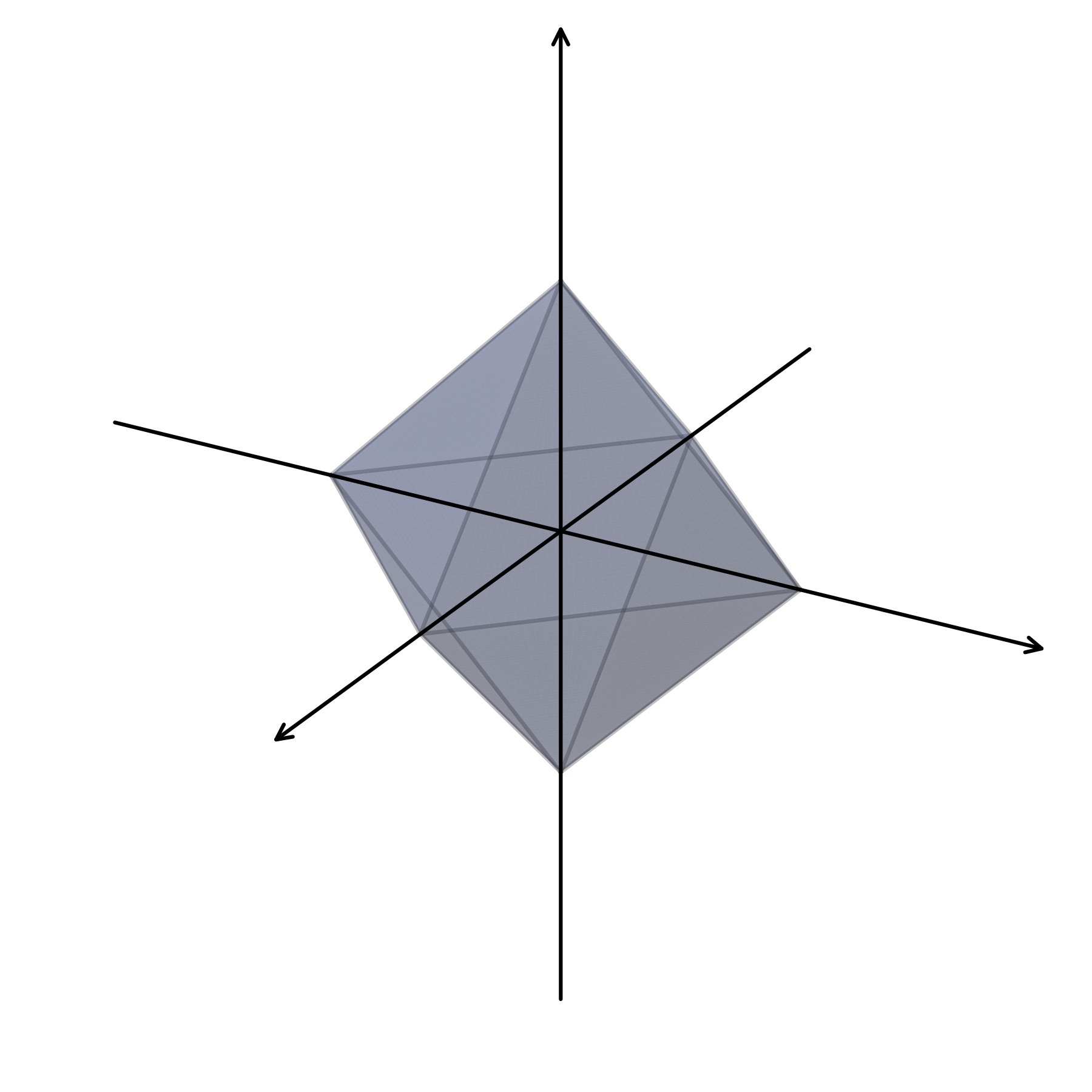
The geometry of the \(\ell_1\) norm directly explains why the Product Laplace distribution induces sparsity. Unlike the smooth \(\ell_2\) sphere, the \(\ell_1\) geometry has sharp corners along coordinate axes, biasing samples toward configurations where many coordinates are small or close to zero. Thus regularizing feature distributions towards product Laplace lead to axis-aligned, sparse representations, while also encourages maximum spreading and hence prevent feature collapse.
The other way to think about why Laplace induces sparsity is through the lens of regularized linear regression. It’s well known that Lasso regression with $\ell_1$ penalty on the weight is equivalent to Maximum A Posteriori (MAP) estimation with a Laplace prior, whereas Ridge regression with $\ell_2$ regularization on the weight corresponds to MAP estimation with a Gaussian prior
Generalized Gaussian Distributions
We observe that both Laplace and Gaussian are maximum-entropy distributions over either expected \(\ell_1\) amd \(\ell_2\) norm constraints. Since the \(\ell_1\)-norm already promotes sparsity, a natural question is how much further can we go.
To answer this, we need to define our sparsity metrics. The most direct notion of sparsity is the $\ell_0$ (pseudo-)norm which simply counts the number of nonzero entries in a vector. However, direct minimization of $\ell_0$ norm is an NP-hard problem
More generally, $\ell_p$ quasi-norms with $0 < p < 1$ provide a closer approximation to $\ell_0$. Their sharp singularity near zero strongly encourages exact sparsity, while their weaker growth for large values reduces shrinkage on important components. Although nonconvex, such penalties are well known to yield significantly sparser representations than $\ell_1$ in practice
Thus we would like to consider distributions with the \(\ell_p\) quasi-norms constraints. In fact, the maximum-entropy distribution under the expected \(\ell_p\)-norm constraints is the zero-mean product Generalized Gaussian distributions \(\prod_{i=1}^{d}\mathcal{GN}_p(\mu,\sigma)\), of which product Laplace and isotropic Gaussian are special cases for \(p=1\) and \(p=2\) respectively.
Probability Density Functions of Product Generalized Gaussian
\[\begin{aligned} p(\mathbf{z}) &= \prod_{i=1}^{d}\frac{p^{1-1/p}}{2\sigma\Gamma(1/p)} \exp\!\left(-\frac{|\mathbf{z}_i-\mu|^p}{p\sigma^p}\right) \\ &= \frac{p^{d-d/p}}{(2\sigma)^d\Gamma(1/p)^d} \exp\!\left(-\frac{\|\mathbf{z}-\boldsymbol{\mu}\|_p^p}{p\sigma^p}\right) \end{aligned}\]
Assume that $\mu=0$ and let \(\mathbf{z}\sim\prod_{i=1}^{d}\mathcal{GN}_p(\mu,\sigma)\). Then the radius \(r^p:=\|\mathbf{z}\|_p^p\sim\Gamma(d/p,p\sigma^p)\) follows the Gamma distribution and the angular direction \(\mathbf{u}:=\mathbf{z}/\|\mathbf{z}\|_p\) follows the cone measure on the $\ell_p$ sphere \(\mathbb{S}^{d-1}_{\ell_{p}}:=\{\mathbf{z}\in\mathbb{R}^d\mid\|\mathbf{z}\|_p=1\}\) with the radial-angular independence \(r\perp \!\!\ \mathbf{u}\)
Details on Cone and Surface Measure
The cone measure is identical to the \((d-1)\)-dimensional Hausdorff measure \(\mathcal{H}^{d-1}\) (also called surface measure) when \(p\in\{1,2,\infty\}\)
Thus the angular directions of product Laplace and isotropic Gaussian are uniformly distributed over the \(\ell_p\) sphere with respect to the surface measures, whereas any other Generalized Gaussian distributions have angular direction uniform under the cone measure.
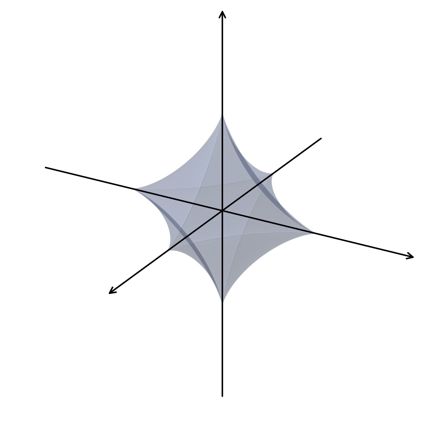
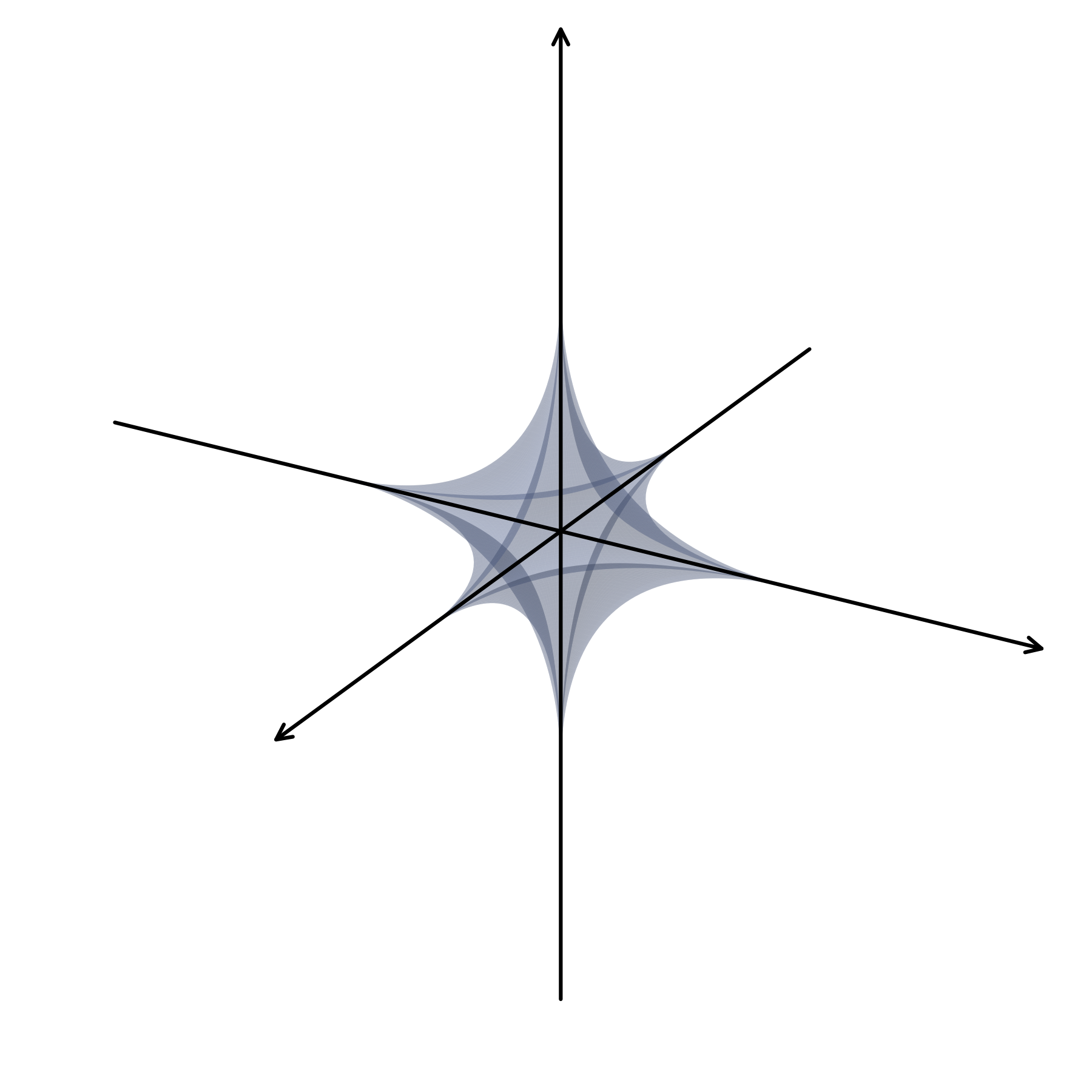
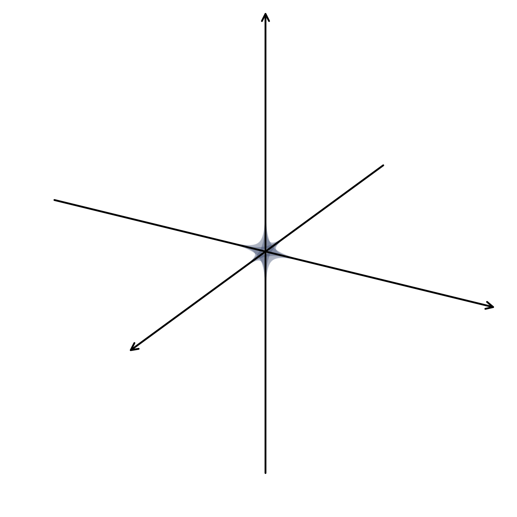
Thus we can always regularizes our feature distributions towards the Generalized Gaussian Distributions \(\prod_{i=1}^{d}\mathcal{GN}_p(\mu,\sigma)\) with \(0<p<1\) for learning even sparser, axis-aligned representations while also preserving the maximum-entropy guarantee to prevent feature collapse.
We denote the family of methods using Eq. (6) with the target distributions being Generalized Gaussian \(\prod_{i=1}^{d}\mathcal{GN}_p(0,\sigma)\) as LpJEPA. When \(p=2\), LpJEPA reduce to LeJEPA since the target distribution becomes the isotropic Gaussian.
Rectified Generalized Gaussian Distributions (RGG)
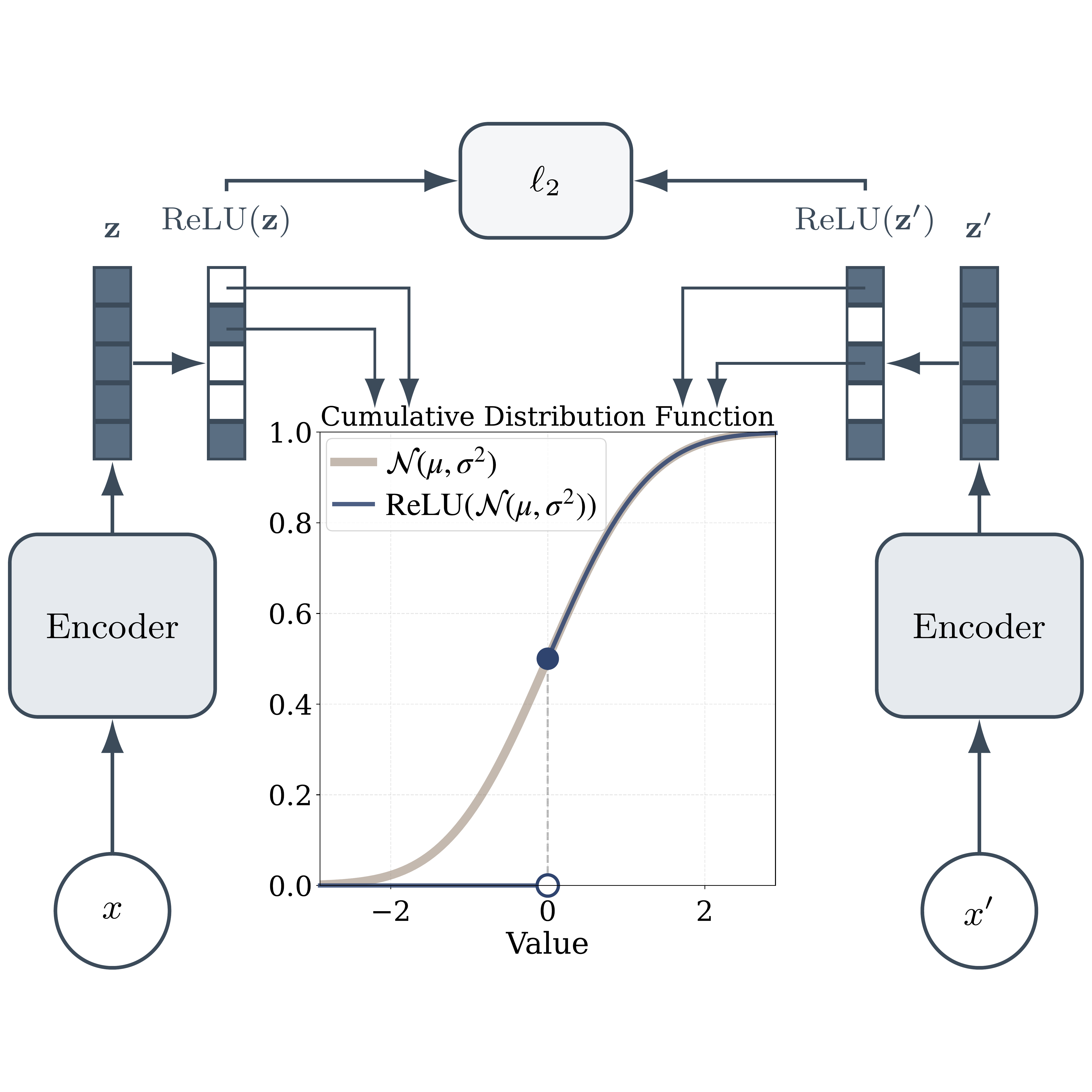
The Generalized Gaussian family is a well-known distribution, but we’re not satisfied with the \(\ell_p\)-norm sparsity it induces. In fact, it’s possible to directly encode \(\ell_0\)-norm into the target distribution, and this brings us to the key innovation of our paper: regularizing rectified features towards the Rectified Generalized Gaussian distributions.
Let \(\mathbf{x}\sim\prod_{i=1}^d\mathcal{GN}_p(\mu,\sigma)\) be a Generalized Gaussian random vector. Then we can obtain the (product) Rectified Generalized Gaussian random vector as \(\mathbf{z}\sim\prod_{i=1}^d\operatorname{ReLU}(\mathcal{GN}_p(\mu,\sigma))\), where we apply the rectifying nonlinearities coordinate-wise to the Generalized Gaussian random vector. We visualize the samples drawn from the Generalized Gaussian and Rectified Generalized Gaussian distribution in \(2\)-dimensions when \(p=2\).
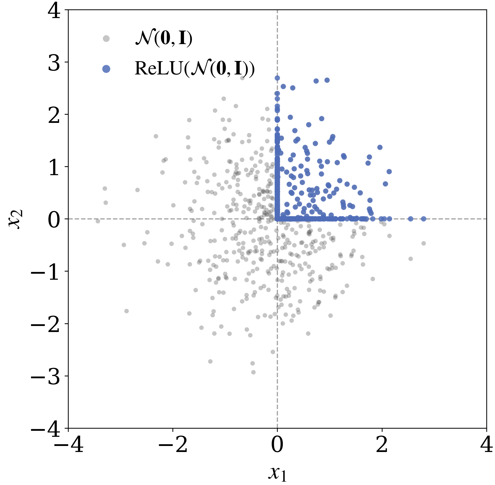
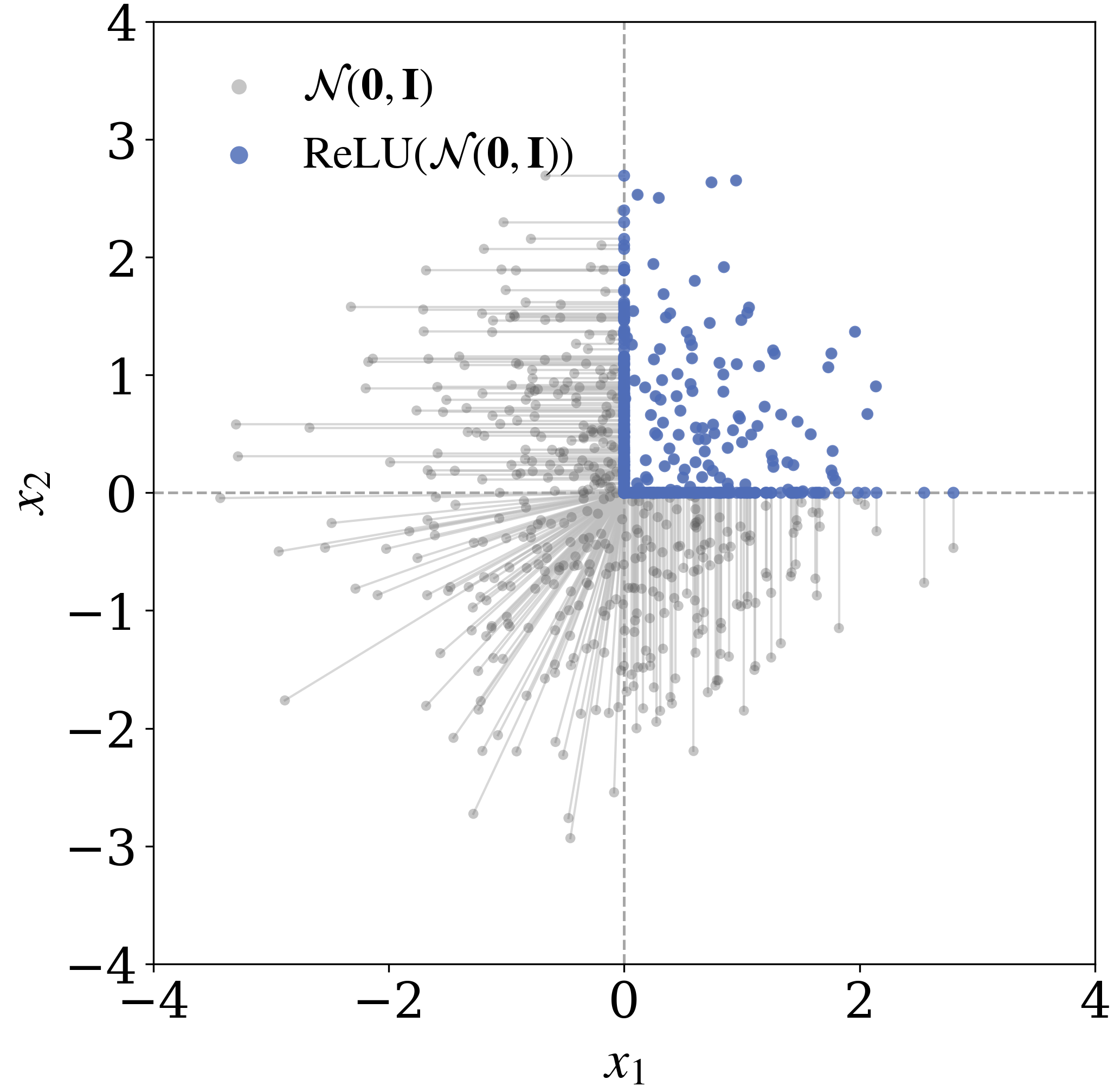
As illustrated in the figure above, rectification collapses all samples lying outside the positive orthant onto its boundary, while samples in the interior of the positive orthant remain unchanged.
Let \(\Phi_{\mathcal{GN}_p(0,1)}\) be the cumulative distribution function for the standard Generalized Gaussian distribution \(\mathcal{GN}_p(0, 1)\). In \(d\)-dimensional spaces, the probability of a Rectified Generalized Gaussian random vector being in the interior of the positive orthant $[0,\infty)^d$ is $(1-\Phi_{\mathcal{GN}_p(0,1)}(-\mu/\sigma))^d$, which decays to $0$ exponentially fast as $d\to\infty$. Thus in high dimensions, most of the rectified samples concentrates on the boundary of the positive orthant cone.
It’s also possible to characterize the probability density function \(f_{\mathcal{RGN}_p(\mu,\sigma)}(\cdot)\) of the univariate Rectified Generalized Gaussian distribution (which we also denote as \(\mathcal{RGN}_p(\mu,\sigma)\)):
\[\begin{align} f_{\mathcal{RGN}_p(\mu,\sigma)}(z)&=\Phi_{\mathcal{GN}_p(0,1)}\bigg(-\frac{\mu}{\sigma}\bigg)\cdot\mathbb{1}_{\{0\}}(z)\tag{8}\\&+\frac{p^{1-1/p}}{2\sigma\Gamma(1/p)}\exp\bigg(-\frac{|z-\mu|^p}{p\sigma^p}\bigg)\cdot\mathbb{1}_{(0,\infty)}(z)\tag{9} \end{align}\]where \(\Gamma(\cdot)\) is the Gamm function and \(\mathbb{1}_{S}(z)\) is the indicator function that evaluates to \(1\) if \(z\in S\) and \(0\) otherwise. We note the the probability density function here is in fact the Radon-Nikodym derivative of the Rectified Generalized Gaussian probability measure with respect to the Dirac + Lebesgue measure. Further details can be found in the paper.
Measure-Theoretical Characterizations of the Rectified Generalized Gaussian Distribution
Fix parameters \(p>0\), \(\mu\in\mathbb{R}\), and \(\sigma>0\). We denote \((\mathbb{R}, \mathcal{B}(\mathbb{R}))\) as the real line equipped with Borel \(\sigma\)-algebra. Let \(\lambda\) be the Lebesgue measure on \(\mathcal{B}(\mathbb{R})\) and let \(\delta_0\) be the Dirac measure at \(0\). The probability measure \(\mathbb{P}_{X}\) of the Rectified Generalized Gaussian random variable \(X\) is given by the mixture
\[\mathbb{P}_{X}=\Phi_{\mathcal{GN}_p(0,1)}\bigg(-\frac{\mu}{\sigma}\bigg)\cdot\delta_0+\bigg(1-\Phi_{\mathcal{GN}_p(0,1)}\bigg(-\frac{\mu}{\sigma}\bigg)\bigg)\cdot\mathbb{P}_{\mathcal{TGN}_p(\mu,\sigma)}\]where \(\mathbb{P}_{\mathcal{TGN}_p(\mu,\sigma)}\) is the Truncated Generalized Gaussian probability measure and \(\Phi_{\mathcal{GN}_p(0,1)}\) is the CDF of the standard Generalized Gaussian \(\mathcal{GN}_{p}(0,1)\).
Define the mixed measure \(\nu:=\lambda+\delta_0\). The Radon-Nikodym derivative of \(\mathbb{P}_X\) with respect to \(\nu\) exists and is given by
\[\frac{d\mathbb{P}_{X}}{d\nu}(x)=f_{\mathcal{RGN}_p(\mu,\sigma)}(x)\]Intuitively, the Rectified Generalized Gaussian distribution can also be viewed as a mixture between a discrete Dirac measure \(\delta_0(x)\) and a Truncated Generalized Gaussian distribution \(\mathcal{TGN}_{p}(\mu,\sigma,(0,\infty))\), where \(\mathcal{TGN}_{p}(\mu,\sigma,(0,\infty))\) has the density function
\[\begin{align} f_{\mathcal{TGN}_{p}(\mu, \sigma, (0,\infty))}(z)=\frac{\mathbb{1}_{(0,\infty)}(z)}{Z_S(\mu,\sigma,p)}\exp\bigg(-\frac{|z-\mu|^p}{p\sigma^p}\bigg) \tag{10} \end{align}\]Sparsity and Entropy Characterizations of RGG
In our paper, we show that if \(\mathbf{x}\sim\prod_{i=1}^{d}\mathcal{RGN}_p(\mu,\sigma)\) in \(d\) dimension, then
\[\begin{align} \mathbb{E}[\|\mathbf{x}\|_0]&=d\cdot\Phi_{\mathcal{GN}_p(0,1)}\bigg(\frac{\mu}{\sigma}\bigg)\tag{11}\\ &=\frac{d}{2}\bigg(1+\operatorname{sgn}\bigg(\frac{\mu}{\sigma}\bigg)P\bigg(\frac{1}{p},\frac{|\mu/\sigma|^p}{p}\bigg)\bigg)\tag{12} \end{align}\]where \(\operatorname{sgn}(\cdot)\) is the sign function and \(P(\cdot,\cdot)\) is the lower regularized gamma function. Thus it’s possible to directly control the expected \(\ell_0\) norm of the Rectified Generalized Gaussian random vector through specifying the set of parameters \(\{\mu,\sigma,p\}\).
Due to rectifications, the RGG distribution is also no longer absolutely continuous with respect to the Lebesgue measure, rendering differential entropy ill-defined. Thus we resort to the concept of \(d(\boldsymbol{\xi})\)-dimensional entropy
Details on \(d(\boldsymbol{\xi})\)-dimensional entropy
Let \(\boldsymbol{\xi}\sim\prod_{i=1}^{D}\mathcal{RGN}_p(\mu,\sigma)\) be a Rectified Generalized Gaussian random vector. The Rényi information dimension of \(\boldsymbol{\xi}\) is \(d(\boldsymbol{\xi})=D\cdot\Phi_{\mathcal{GN}_p(0,1)}(\mu/\sigma)\), and the \(d(\boldsymbol{\xi})\)-dimensional entropy of \(\boldsymbol{\xi}\) is given by
\[\begin{align} \mathbb{H}_{d(\boldsymbol{\xi}_i)}(\boldsymbol{\xi}_i)&=\Phi_{\mathcal{GN}_p(0,1)}\bigg(\frac{\mu}{\sigma}\bigg)\cdot\mathbb{H}_{1}(\mathcal{TGN}_p(\mu,\sigma))\tag{*}\\ &+\mathbb{H}_{0}(\mathbb{1}_{(0,\infty)}(\boldsymbol{\xi}_i))\tag{*}\\ \mathbb{H}_{d(\boldsymbol{\xi})}(\boldsymbol{\xi})&=\sum_{i=1}^{D}\mathbb{H}_{d(\boldsymbol{\xi}_i)}(\boldsymbol{\xi}_i)=D\cdot \mathbb{H}_{d(\boldsymbol{\xi}_i)}(\boldsymbol{\xi}_i)\tag{*} \end{align}\]where \(\mathbb{H}_0(\cdot)\) is the discrete Shannon entropy, \(\mathbb{H}_1(\cdot)\) denotes the differential entropy, and \(\mathbb{1}_{(0,\infty)}(\boldsymbol{\xi}_i)\) is a Bernoulli random variable that equals \(1\) with probability \(\Phi_{\mathcal{GN}_p(0,1)}(\mu/\sigma)\) and \(0\) with probability \(1-\Phi_{\mathcal{GN}_p(0,1)}(\mu/\sigma)\).
Thus we choose the Rectified Generalized Gaussian as our target distribution \(Q\), which has an explicit expected \(\ell_0\) norm guarantees, while also preserve the maximum-entropy property under the expected \(\ell_p\) norm constraint under rescaling. The distribution-matching loss towards the Rectified Generalized Gaussian family is called Rectified Distribution Matching Regularization (RDMReg), and a Joint-Embedding Predictive Architecture (JEPA) equipped with RDMReg is called Rectified LpJEPA. We dive into these two things in the rest of this blog post.
Rectified Distribution Matching Regularization (RDMReg)
After identifying the desirable target distribution as the Rectified Generalized Gaussian family, we would like to regularize the neural network feature towards it using Eq. (6).
Contrary to the isotropic Gaussian, which is closed under linear combinations, the Rectified Generalized Gaussian (RGG) family is not preserved under linear projections: the one-dimensional projected marginals generally fall outside the RGG family. In fact, closure under linear combinations characterizes the class of multivariate stable distributions
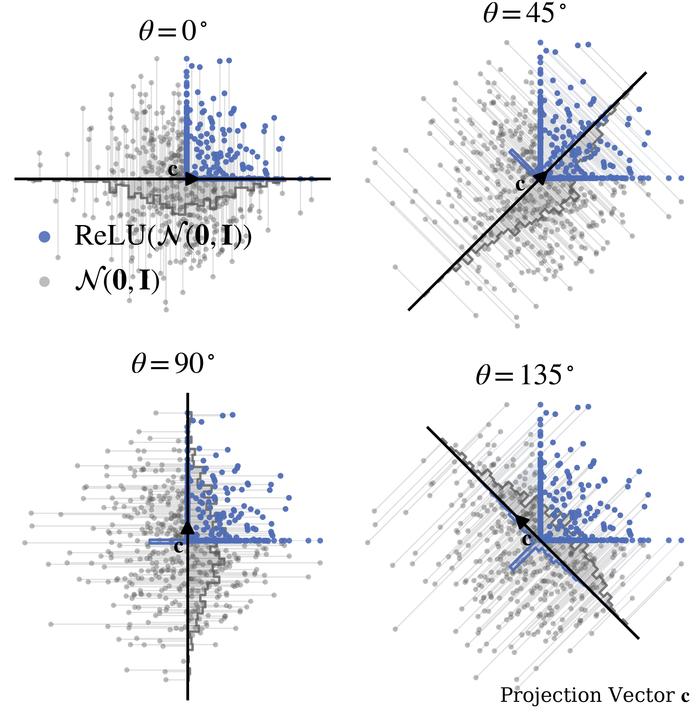
Consequently, the distribution matching loss \(\mathcal{L}(\cdot\|\cdot)\) must rely on sample-based, nonparametric two-sample hypothesis tests on projected marginals
Let \(\mathbf{Z},\mathbf{Y}\in\mathbb{R}^{B\times D}\) be empirical neural network feature matrix and the samples from RGG where \(B\) is batch size and \(D\) is dimension. We denote a single random projection vector as \(\mathbf{c}_i\in\mathbb{R}^D\) out of \(N\) total projections.
The Rectified Distribution Matching Regularization (RDMReg) loss function is given by
\[\begin{align} \mathcal{L}_{\operatorname{RDMReg}}(\mathbb{P}_{\mathbf{c}_i^\top\mathbf{z}}\|\mathbb{P}_{\mathbf{c}_i^\top\mathbf{y}}):=\frac{1}{B}\|(\mathbf{Z}\mathbf{c}_i)^{\uparrow}-(\mathbf{Y}\mathbf{c}_i)^{\uparrow}\|_2^2\tag{13} \end{align}\]where \((\cdot)^{\uparrow}\) denotes sorting in ascending order. The objective is implemented in the following python code snippet
import torch

def rdmreg_loss(z, target_samples, num_projections):
    B, D = z.shape
    device = z.device

    # 1. Sample random projections from the unit L2 sphere.
    projections = torch.randn(num_projections, D, device=device)
    projections = projections / projections.norm(dim=1, keepdim=True)

    # 2. Project features and samples from the RGG distribution.
    proj_z = torch.matmul(z, projections.T)
    proj_target = torch.matmul(target_samples, projections.T)

    # 3. Sort along the batch dimension
    proj_z_sorted, _ = torch.sort(proj_z, dim=0)
    proj_target_sorted, _ = torch.sort(proj_target, dim=0)

    # 4. Compute and Return the Sliced 2-Wasserstein distance
    return torch.mean((proj_z_sorted - proj_target_sorted)**2)
Rectified LpJEPA
Equipped with RDMReg, we arrive at our final objective function
\[\begin{align} \min_{\boldsymbol{\theta}}\mathbb{E}_{\mathbf{z},\mathbf{z}'}[\|\mathbf{z}-\mathbf{z}'\|_2]&+\mathbb{E}_{\mathbf{c}}[\mathcal{L}_{\operatorname{RDMReg}}(\mathbb{P}_{\mathbf{c}^\top\mathbf{z}}\|\mathbb{P}_{\mathbf{c}^\top\mathbf{y}})]\tag{14}\\&+\mathbb{E}_{\mathbf{c}}[\mathcal{L}_{\operatorname{RDMReg}}(\mathbb{P}_{\mathbf{c}^\top\mathbf{z}'}\|\mathbb{P}_{\mathbf{c}^\top\mathbf{y}})]\tag{15} \end{align}\]where \(\mathbf{y}\sim\prod_{i=1}^{d}\mathcal{RGN}_{p}(\mu,\sigma)\) is a Rectified Generalized Gaussian random vector and \(\mathbf{z}=f_{\boldsymbol{\theta}}(\mathbf{x})\), \(\mathbf{z}'=f_{\boldsymbol{\theta}}(\mathbf{x}')\) are the neural network features.
In standard self-supervised learning protocols
In contrast, we explicitly introduce an additional rectification at the output and we arrive at: \(\mathbf{z} = f_{\boldsymbol{\theta}}(\mathbf{x})= \operatorname{ReLU}\!\left(g_{\boldsymbol{\theta}_2}\bigl(g_{\boldsymbol{\theta}_1}(\mathbf{x})\bigr)\right).\) This final \(\operatorname{ReLU}(\cdot)\) is a deliberate architectural choice and is essential for the correctness of our method. Combining the architectural and objective-level updates, we arrive at Rectified LpJEPA.
Sparsity-Performance Tradeoffs
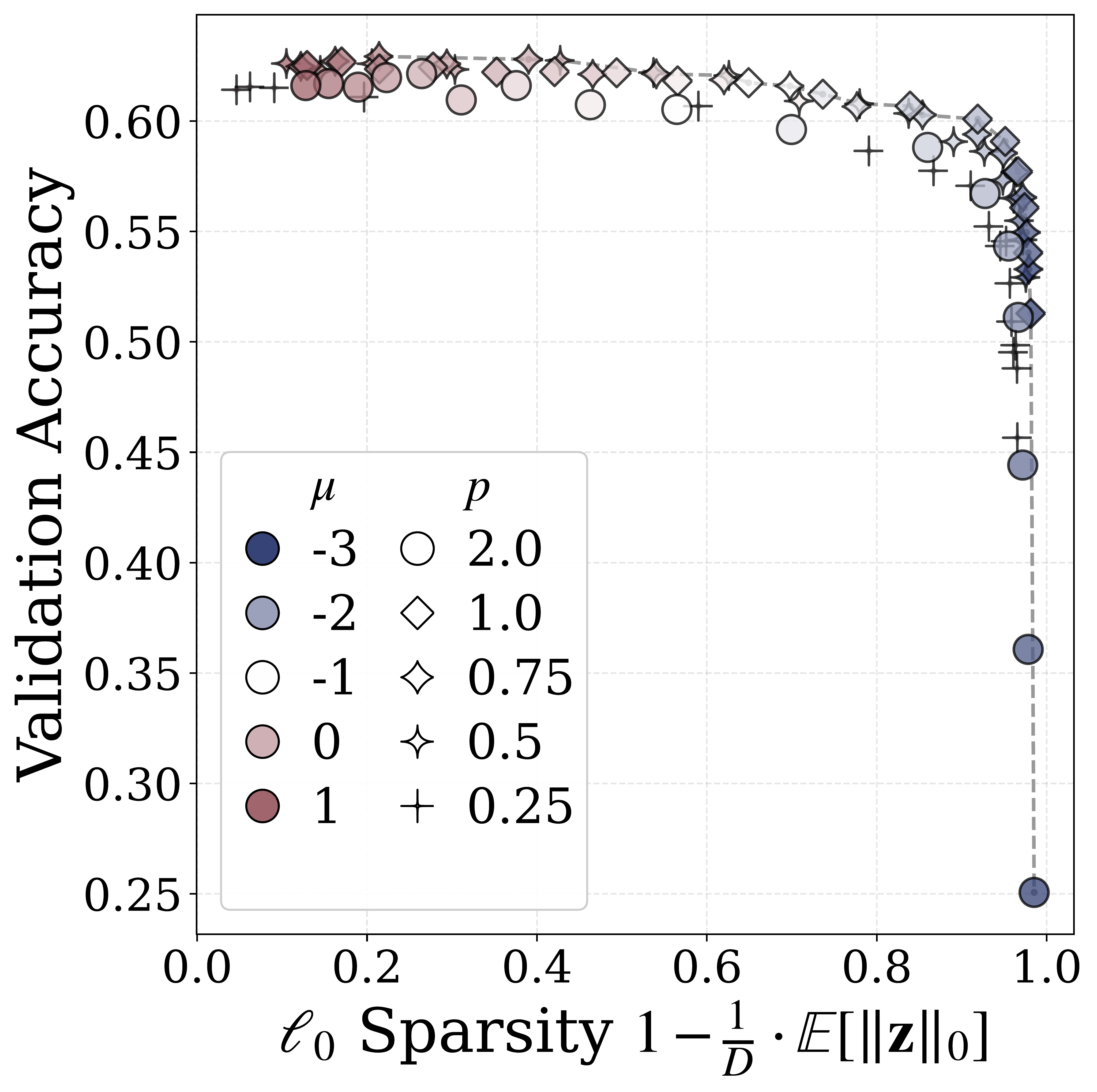
Finally, we can train our Rectified LpJEPA model. For simplicity, we can consider self-supervised pretraining over the CIFAR-100 dataset. By varying the mean shift values \(\mu\) and the \(\ell_p\) parameter \(p\) while fixing \(\sigma=\Gamma(1/p)^{1/2}/(p^{1/p}\cdot\Gamma(3/p)^{1/2})\), we observe a clear sparsity-performance tradeoff
More experiments and ablation studies can be found in the paper. Overall, Rectified LpJEPA provides a principled approach to learning sparse representations through distribution matching to Rectified Generalized Gaussian. If you find this work useful, please consider checking out the paper and codebase and citing our work:
@misc{kuang2026rectifiedlpjepajointembeddingpredictive,
      title={Rectified LpJEPA: Joint-Embedding Predictive Architectures with Sparse and Maximum-Entropy Representations},
      author={Yilun Kuang and Yash Dagade and Tim G. J. Rudner and Randall Balestriero and Yann LeCun},
      year={2026},
      eprint={2602.01456},
      archivePrefix={arXiv},
      primaryClass={cs.LG},
      url={https://arxiv.org/abs/2602.01456},
}